SensibleAI Studio: ML Regression 101

Author: Graham Eger, Created: 2025-02-28

What is Regression?

Machine learning regression is a predictive analytics technique that helps organizations forecast numerical outcomes by modeling relationships between a dependent variable (the target) and one or more independent variables (features). Unlike clustering, which groups similar data points, regression predicts continuous values such as sales revenue, expenses, or other financial metrics. A common example is predicting next quarter’s revenue based on historical sales data, marketing spend, and economic indicators.

How does it work?

To understand regression, let's start with a simple example. Suppose a company wants to predict monthly sales based on its advertising spend. Using Linear Regression, one of the simplest regression techniques, the algorithm plots historical advertising spend (feature) against monthly sales (target). The goal is to fit a straight line that minimizes the total squared difference between actual sales and predicted sales.

Initially, the algorithm makes an estimate (the regression line) based on existing data. It then iteratively adjusts the line to reduce errors (distance between predicted and actual sales) until it finds the line that best fits the data. The result is a mathematical function that clearly shows how changes in advertising spend directly affect sales.

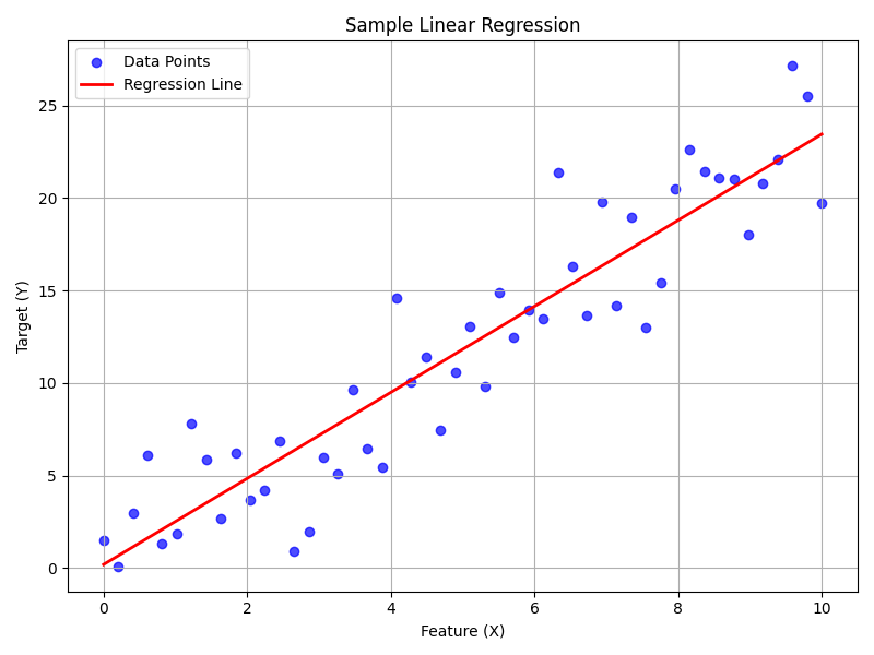
Sample Linear Regression Plot source code

import numpy as np
import matplotlib.pyplot as plt

# Generate sample data
np.random.seed(42)
x = np.linspace(0, 10, 50)
y = 2.5 * x + np.random.normal(0, 3, 50)

# Perform manual linear regression calculations
coefficients = np.polyfit(x, y, 1)
y_pred = coefficients[0] * x + coefficients[1]

# Plot the data points and the regression line
plt.figure(figsize=(8, 6))
plt.scatter(x, y, color='blue', alpha=0.7, label='Data Points')
plt.plot(x, y_pred, color='red', linewidth=2, label='Regression Line')

# Titles
plt.title('Sample Linear Regression')
plt.xlabel('Feature (X)')
plt.ylabel('Target (Y)')
plt.legend()
plt.grid(True)

# Show plot
plt.tight_layout()
plt.show()

What are common types of machine learning regression?

While Linear Regression is straightforward and interpretable, real-world scenarios often require more sophisticated methods. Popular advanced techniques include:

• Decision Trees: These models partition data into subsets based on feature values, allowing predictions to be made by following a path of decisions. Decision trees handle non-linear relationships and interactions between variables effectively.

• Random Forests: An ensemble method that builds multiple decision trees and combines their predictions. This reduces overfitting, increases accuracy, and captures complex patterns.

• Gradient Boosting Machines (GBM): GBM sequentially builds and improves weak models (often trees) to form a strong predictive model. It is particularly powerful for scenarios with many interacting features and complex relationships.

• Logistic Regression: Used primarily for classification problems, logistic regression predicts categorical outcomes (such as yes/no, true/false). It calculates the probability of an outcome by applying a logistic function, making it suitable for binary classification scenarios like determining if a customer will churn or whether an email is spam.

• XGBoost Regression: A powerful ensemble method using gradient-boosted decision trees, XGBoost excels in predictive accuracy, especially when modeling complex or non-linear relationships. In the provided example, XGBoost accurately captures the underlying non-linear trend of the data—demonstrating its effectiveness in situations where relationships between variables aren't easily captured by simpler methods like linear regression. This makes it particularly suitable for financial forecasting, customer behavior prediction, and other scenarios involving intricate data patterns.

Logistic Regression

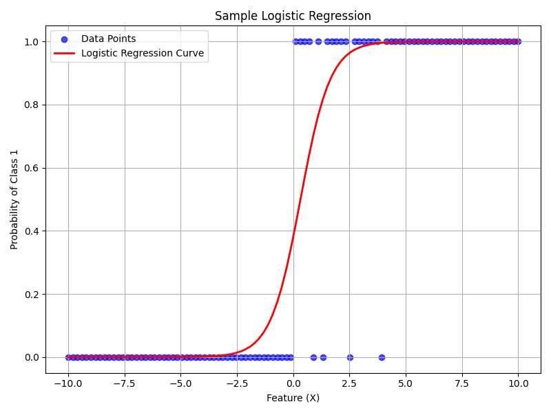
Sample Logistic Regression Plot source code

import numpy as np
import matplotlib.pyplot as plt

# Generate sample binary classification data
np.random.seed(42)
x = np.linspace(-10, 10, 100)
# Sigmoid function
def sigmoid(z):
    return 1 / (1 + np.exp(-z))

# True parameters for synthetic data
true_slope = 1.0
true_intercept = -1.5

# Generate probabilities and binary outcomes
probabilities = sigmoid(true_slope * x + true_intercept)
y = np.random.binomial(1, probabilities)

# Perform logistic regression using numpy (gradient descent manually simplified)
from scipy.optimize import curve_fit

# Logistic function
def logistic(x, a, b):
    return sigmoid(a * x + b)

# Fit logistic regression curve
params, _ = curve_fit(logistic, x, y)
y_pred = logistic(x, *params)

# Plot data and logistic curve
plt.figure(figsize=(8, 6))
plt.scatter(x, y, color='blue', alpha=0.7, label='Data Points')
plt.plot(x, y_pred, color='red', linewidth=2, label='Logistic Regression Curve')

# Customizing plot
plt.title('Sample Logistic Regression')
plt.xlabel('Feature (X)')
plt.ylabel('Probability of Class 1')
plt.legend()
plt.grid(True)

# Display plot
plt.tight_layout()
plt.show()

XGBoost Regression

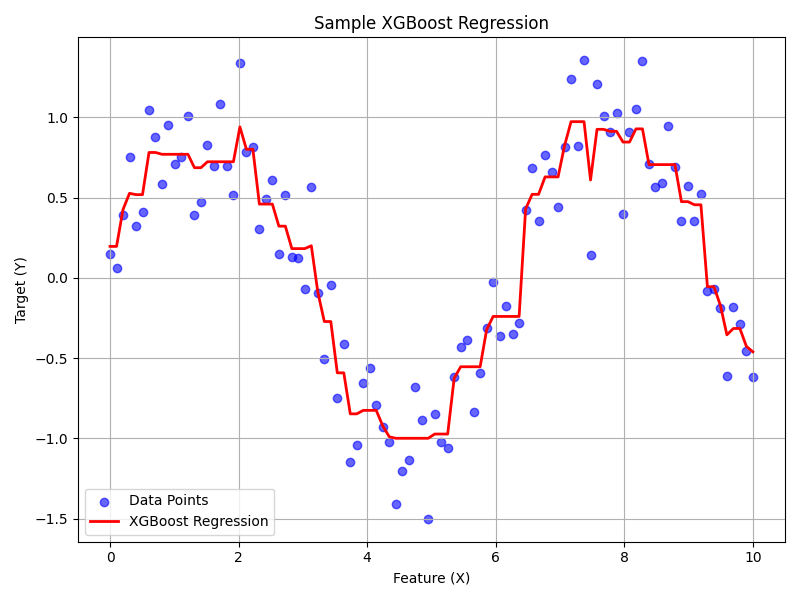
Sample XGBoost Plot source code

import numpy as np
import matplotlib.pyplot as plt
import xgboost as xgb

# Generate sample data
np.random.seed(42)
x = np.linspace(0, 10, 100)
y = np.sin(x) + np.random.normal(0, 0.3, 100)

# Prepare data for XGBoost
X = x.reshape(-1, 1)
dmatrix = xgb.DMatrix(X, label=y)

# XGBoost regression parameters
params = {
    'objective': 'reg:squarederror',
    'max_depth': 3,
    'eta': 0.1,
    'seed': 42
}

# Train XGBoost model
model = xgb.train(params, dmatrix, num_boost_round=50)

# Make predictions
y_pred = model.predict(dmatrix)

# Plot the data points and the XGBoost regression predictions
plt.figure(figsize=(8, 6))
plt.scatter(x, y, color='blue', alpha=0.6, label='Data Points')
plt.plot(x, y_pred, color='red', linewidth=2, label='XGBoost Regression')

# Customizing plot
plt.title('Sample XGBoost Regression')
plt.xlabel('Feature (X)')
plt.ylabel('Target (Y)')
plt.legend()
plt.grid(True)

# Display plot
plt.tight_layout()
plt.show()

How do you choose a regression model?

Selecting the right regression model depends on your data, the complexity of relationships, and your need for interpretability versus predictive accuracy. Here's a quick guide:

Linear Regression: Best when you want a simple, explainable relationship and interpretability is crucial.

Decision Trees: Useful when dealing with complex interactions or non-linear relationships but still desiring interpretability.

Random Forest or Gradient Boosting: Ideal for situations demanding high predictive accuracy and where complexity is significant, though they offer less straightforward interpretability.

What is an example of regression in finance?

Consider a financial planning scenario where a company wants to forecast operating expenses. Historical data includes factors such as employee headcount, revenue, marketing spend, and technology expenses. By using regression analysis, the finance team builds a model that accurately predicts future operating expenses based on anticipated changes in these factors.

For example, after analyzing historical data, the model may produce insights like the following:

A 10% increase in headcount leads to an 8% increase in operating expenses; and A 5% increase in revenue typically drives a 2% increase in technology costs.

These insights help management proactively plan budgets, allocate resources, and perform scenario analyses.

How is regression useful for business decisions?

Regression provides a structured approach to understanding financial trends, predicting outcomes, and guiding strategic decisions. It enables organizations to:

• Forecast revenues and costs accurately.

• Identify key cost drivers and revenue influencers.

• Optimize resource allocation by quantifying impacts.

• Conduct scenario analyses to evaluate strategic choices.

By integrating regression models into Corporate Performance Management (CPM) platforms, finance teams can continuously update forecasts, adapt to changing conditions quickly, and ensure data-driven decision-making without the need for deep data science expertise.

Ultimately, machine learning regression transforms raw financial data into actionable insights, empowering organizations to anticipate future trends and make informed, confident decisions.